Completing Capstone: RL Fastest-Path Planning for Stuart

This year I wrapped up my ECE 4600 capstone project: Stuart, the Smart Micromouse Maze Solver. Stuart is an autonomous robot inspired by the IEEE Micromouse competition, where a small robot explores an unknown maze, builds an internal map, finds a route to the goal, and then tries to traverse that route as quickly as possible.

The project ended on a special note, winning the IEEE Winnipeg Section 1st Prize 2026 for the capstone!

Our team was Rodrigo Alegria, Rajdeep Gill, Connor Pagtakhan, Jonah St. Hilaire, and myself. We were advised by Dr. Ahmed Ashraf and Dr. Philip Ferguson, with external support from PTx Trimble.

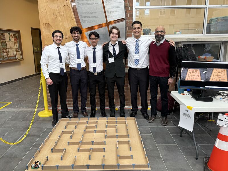
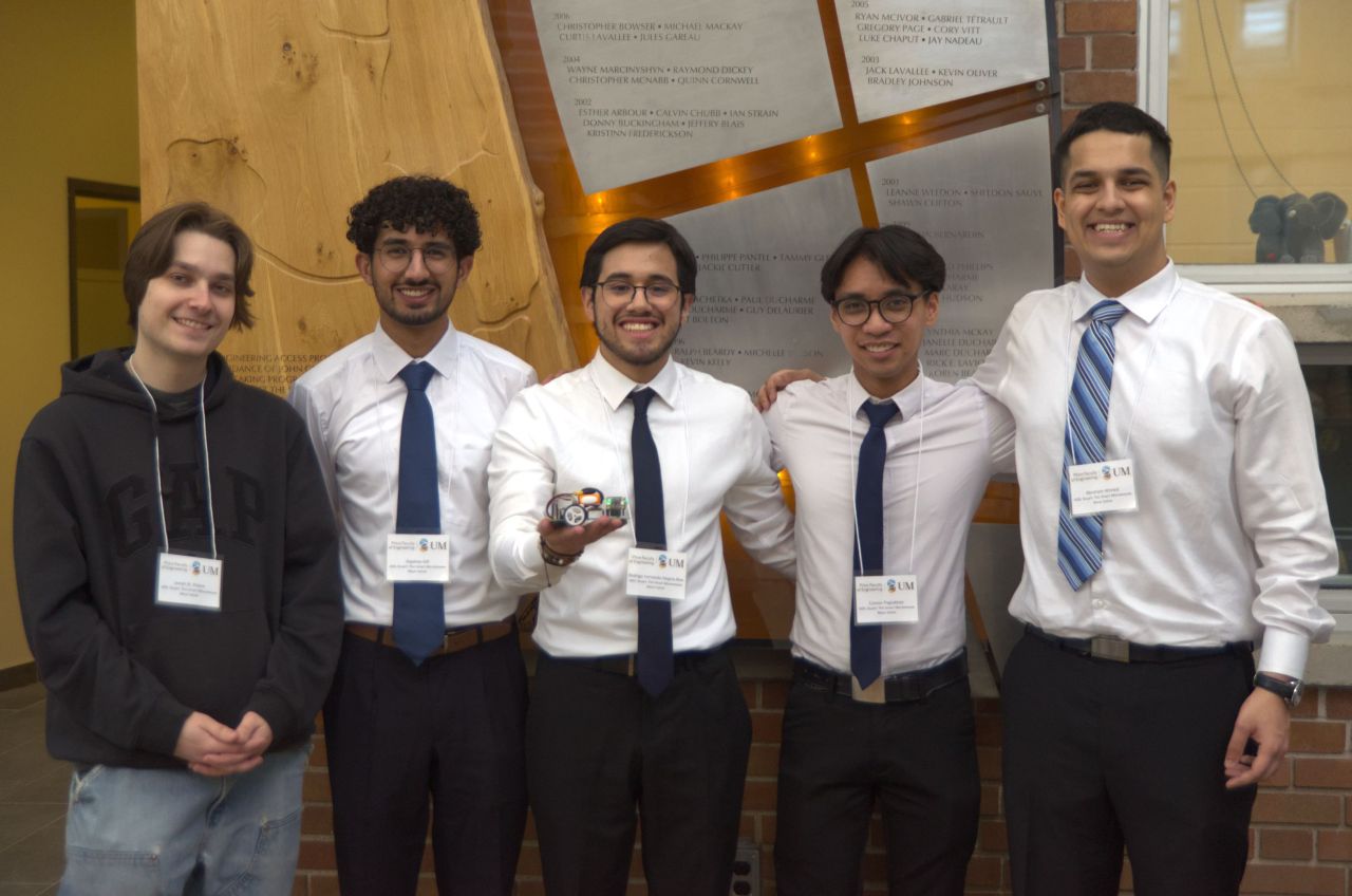Figure 1: Our capstone team with Stuart after the final showcase.

My technical focus was the reinforcement learning / fastest path planning framework. I also led the system architecture and requirements work, but this post is mainly centered on the RL side. The hardware, PCB, low level control, sensing, and deterministic maze exploration work were major teammate-led parts of the project, so I describe them here as system context rather than as my technical deep dive.

Micromouse Context

Micromouse is a robotics challenge where a small autonomous robot must navigate an unknown maze, discover the layout, and reach the centre goal. The robot has two processes: first, explore the maze to build an internal map, and second, use that map to choose a route for the final run. Once the maze is known, the problem can be represented as a graph, where cells are nodes and open passages are edges. At that level, the simplest goal is to find the shortest route from start to goal. However, the robot has to execute turns, accelerate, decelerate, correct its heading, and follow motion commands.

Problem Setup

The planning problem changes significantly depending on the objective used to judge a route. If the goal is only to minimize distance through an unweighted maze graph, then the correct baseline is a deterministic shortest path method: BFS, or equivalently Dijkstra’s algorithm with uniform edge weights. In that view, reinforcement learning is unnecessary because every legal cell transition has the same cost. Our RL formulation instead treated the maze as a fastest traversal problem, where turns, stops, acceleration, command overhead, and long straight segments change the true cost of a path. Under this objective, the shortest route by cell count may not be the fastest route for a physical robot.

Why RL?

A Micromouse maze can be treated as a graph: each cell is a node, and each open wall creates an edge to a neighboring cell. The deterministic baseline solves for the shortest route through that graph. In path form, that is minimizing cell count:

A physical robot takes time to solve a maze during turns, acceleration, deceleration, wheel slip, re-centering, and command overhead. A path with fewer cells may be slower if it forces the robot to stop and rotate repeatedly. A longer path with fewer turns and longer straightaways can win on time.

The objective formulated for time is:

where $\tau$ is the executed trajectory and $\Delta t(a_t)$ is the time cost of the command selected at step $t$.

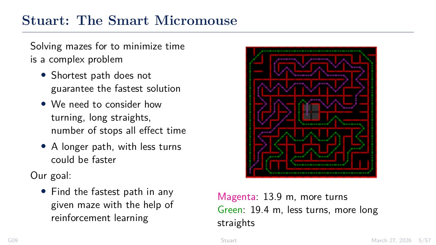Figure 2: Final presentation slide motivating fastest-path planning

So the main question became:

Can a learned policy optimized for shortest time beat a deterministic shortest path baseline?

System Context

The rest of Stuart mattered because the RL planner had to connect to a real robot instead of simulation. The capstone system had three major subsystems: a compact PCB based chassis, an embedded sensing and control stack, and a path optimization layer. The hardware and control work gave the planner executable motion primitives, while the deterministic maze solver provided the explored connectivity map and the Dijkstra shortest path baseline.

For my RL work, I treated those teammate led subsystems as interfaces. The trained policy selected high level actions that could be mapped onto the robot’s command structure: turn, move forward by a number of cells, or stop.

RL Formulation

For the fastest path planning approach, it could be modelled as a Markov Decision Process:

where $\mathcal{S}$ is the state space, $\mathcal{A}$ is the action space, $P$ is the transition model, $r$ is the reward function, and $\gamma$ is the discount factor.

The policy was applied after exploration, so it could assume the maze was fully known. That let the state include both the robot pose and the explored maze structure:

Here:

• $p_t = (x_t, y_t)$ is the robot’s current cell.
• $h_t$ is the heading.
• $o_t = [o_f, o_r, o_b, o_l]$ encodes local motion feasibility.
• $c_t = [c_1, \ldots, c_{k_{\max}}]$ is a forward lookahead vector.
• $w \in \lbrace 0,1 \rbrace^{4N}$ is the flattened maze connectivity map for $N$ cells.

That last term, $w$, is important. Without the full maze map, the policy would be solving a partially observed problem. With the explored connectivity included, the state is much closer to satisfying the Markov property for high level route selection. It isn’t mainly required due to the project scope only having one maze to test, however it is added to eventually train the policy on any general maze in the future.

Simulation Environment

A discrete maze environment was chosen using OpenAI’s Gymnasium, and use of StableBaseline3, rather than a full physics simulator. The simulator tracked Stuart’s cell position, heading, wall connectivity, and goal region. A turn action updated the heading, while a forward action attempted to move the robot by $k$ cells along its current heading:

For a command like $\mathrm{MoveFwd}(k,v)$, the environment checked the next $k$ cell transitions against the maze. If the path was clear, the robot advanced to the new cell and the action contributed a timing cost. If a wall blocked the move, that action was treated as invalid and removed through action masking.

The discrete formulation was intentional so that the learned policy is to stay separated from low level dynamics and produce motion commands for the MCU, such as forward segments and turns. A full physical simulation could also be used to generate these instruction sequences, but it would require additional modeling of turn time, acceleration, deceleration, wheel slip, and controller behaviour. For this project, those parameters were better treated as measurable timing costs that could be estimated from physical testing and folded into the planning objective. As well as for real time debugging purposes, this design decision was kept to have a common communication ground among all subsystems in the project too.

Action Space

The action space was designed to match the embedded command interface:

The forward command is parameterized by distance and speed:

This was one of the most important design choices. The policy was not allowed to invent arbitrary continuous motions. It selected from commands that could be post processed into instructions like:

F 7, R, F 7, R, ...

The use of invalid action masking was also added. If a forward command would cross a wall, that command was masked out before action selection:

That kept learning focused on timing and route selection instead of wasting rollouts on commands that immediately collide with walls.

Reward and Cost

The simplest way to make RL care about speed is to penalize time. The action time model was:

Here $L$ is the maze cell length, $v$ is the selected forward speed, and $t_{\text{turn}}$ is the nominal time cost assigned to a $90^\circ$ turn.

The reward combined a terminal goal reward, time cost, turn cost, and shaping based on progress toward the goal. I used a BFS distance to goal field $d(\cdot)$ for shaping:

A simplified version of the reward is:

The $\min(\delta_t, 2)$ cap was added so that long forward moves helped the agent, but did not create reward spikes so large that training became focused on jumping for strictly long straights.

PPO Training

For the final implementation, I used Maskable PPO with an MLP policy. PPO was a good fit because it is stable enough for iterative reward shaping, and the maskable variant let the environment remove invalid moves without changing the high level action design.

The clipped PPO objective is:

with:

PPO lets the policy improve the probability of actions that produced better than expected returns, while clipping the update so the new policy does not move too aggressively in one step.

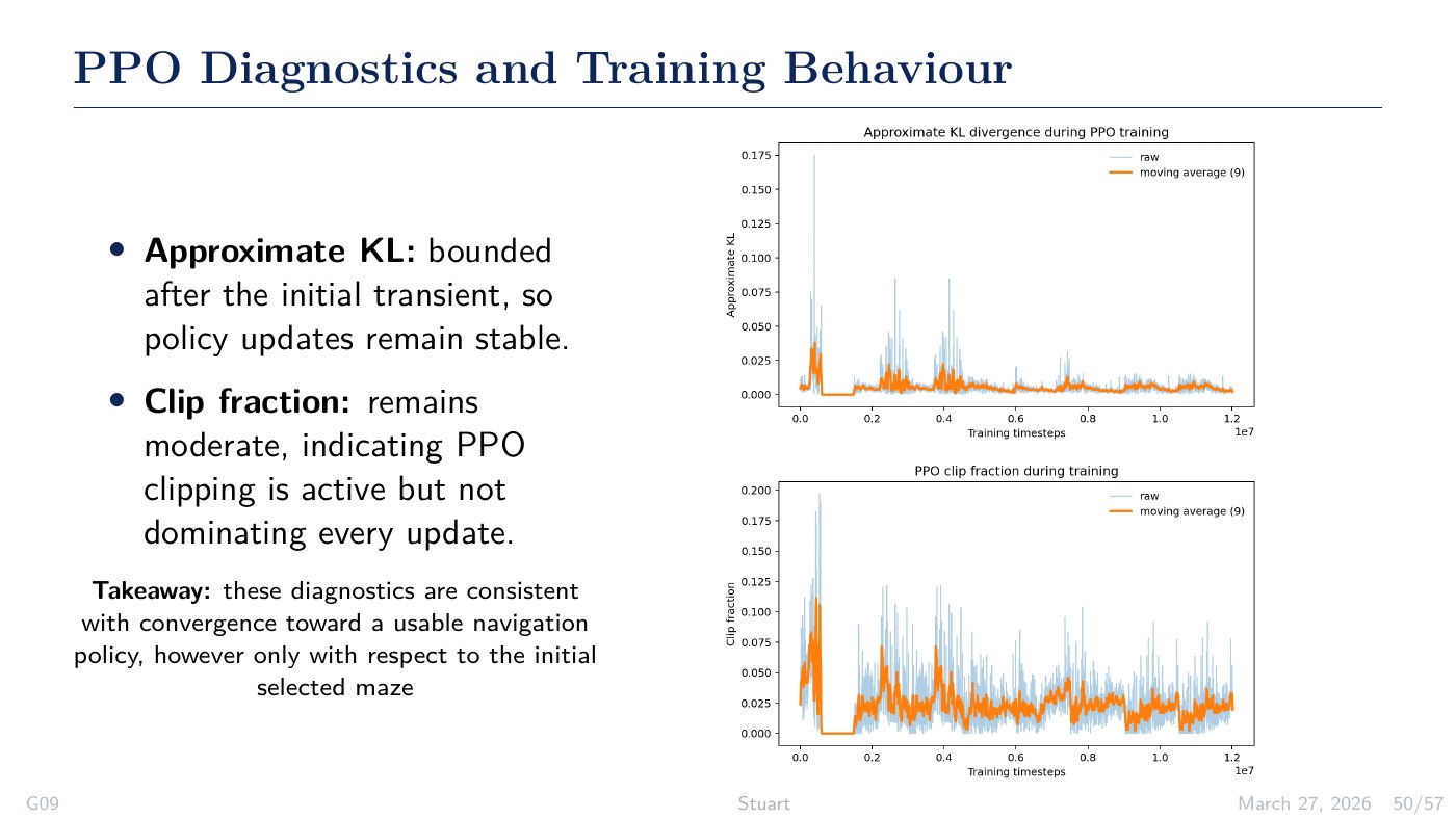Figure 3: PPO diagnostics for the trained navigation policy, showing bounded KL behaviour and moderate clipping.

Policy Export

The trained policy produced raw navigation actions in simulation. Before sending those actions toward hardware, consecutive forward moves were merged into compact instruction sequences:

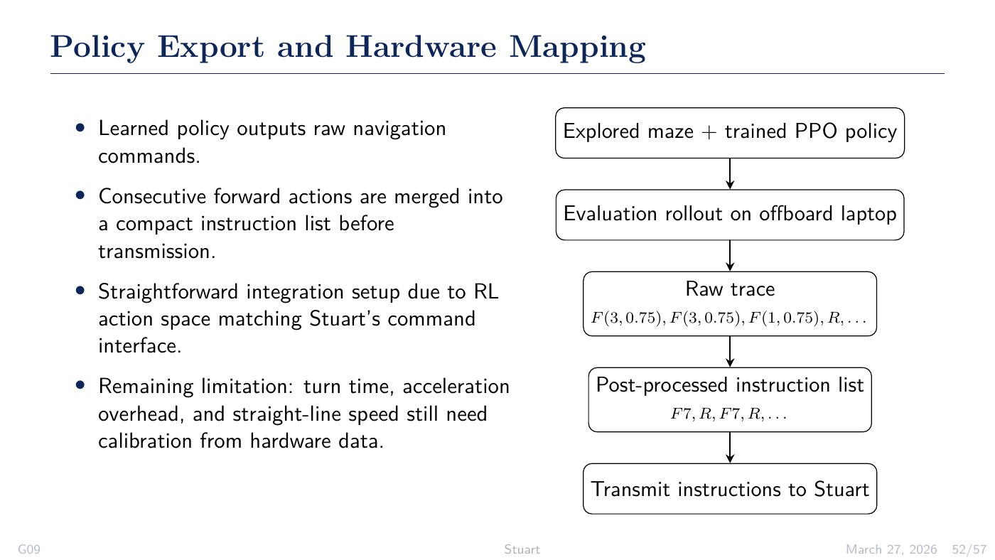Figure 4: Policy export flow converting raw RL actions into compact hardware-style instructions.

This bridge between RL and embedded control was really interesting to see at the final step. A policy that produces shaped commands for the fastest time is super cool to see output everytime.

Result: Longer Path, Faster Time

The main comparison was against Dijkstra’s shortest path from the nominal start state $(0,0)$. We were able to obtain physical times as well for our last sprint!

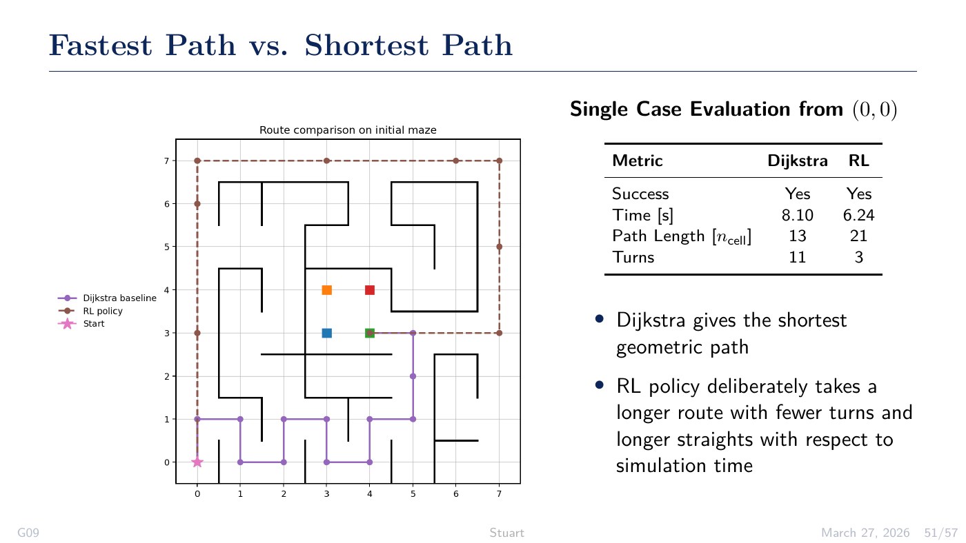Figure 5: Single-case comparison where the RL policy takes a longer route with fewer turns and lower simulated time.

In that evaluation:

• Dijkstra found a 13-cell route with 11 turns and a physical time of 30.264 s
• The RL policy found a 21-cell route with only 3 turns and a physical time of 21.788 s.

You can watch the physical run video here.

The distance ratio was:

The time ratio was:

So the learned route was about 1.62x longer by cell count, but about 28% faster in the physical timing comparison. That directly supported the hypothesis behind the RL work:

when the cost of executing the path is considered.

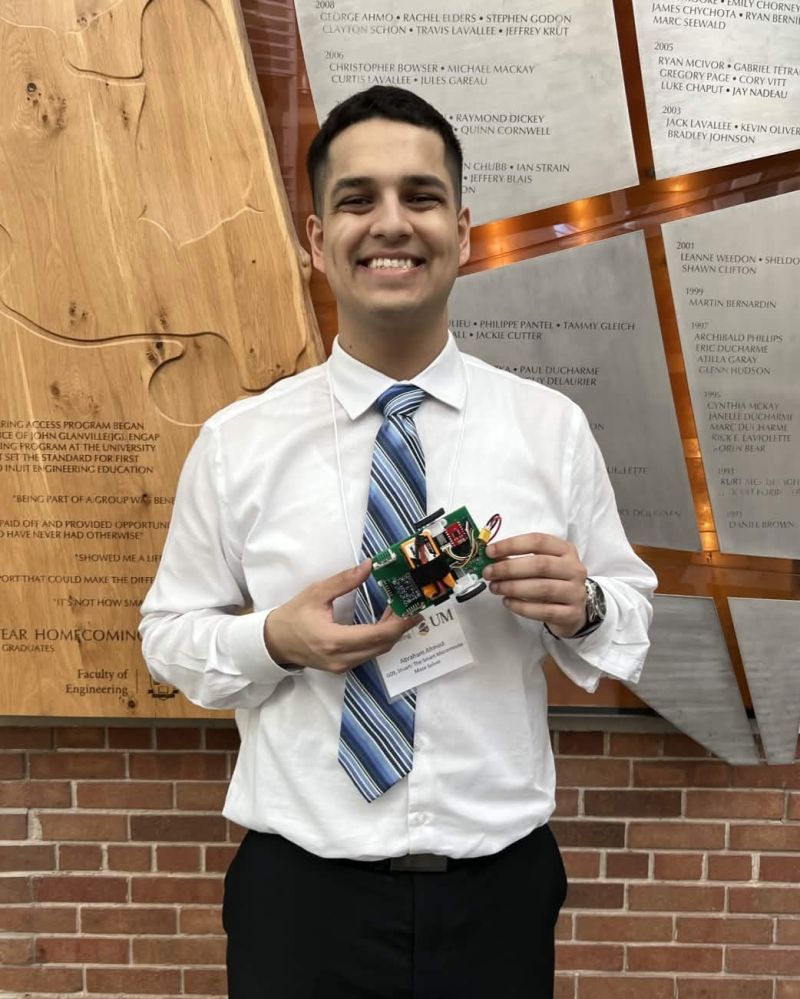Figure 6: Holding Stuart at the capstone showcase after the final demo and testing push.

What I Took Away

The biggest lesson was that RL for robotics was the problem formulation matters a great deal being, what the state includes, what actions are allowed, reward shaping as a whole, and whether the policy output can actually be executed by the robot.

The hardware, sensing, control, deterministic solver, and RL components were each validated and complete end to end physical maze solving still had integration challenges inside the real maze. That limitation is important cause it means the RL result should be read as a fastest path planning result in simulation, based on the robot’s command structure. That is still exactly why I liked this capstone. It made the abstraction boundaries visible. The learned planner depended on a deterministic map. The reward depended on a timing model. The timing model depended on real motion primitives. The motion primitives depended on control and sensing. Every layer of abstraction was in direct need of another, and every layer had assumptions that the next layer either depended on or exposed.

Next Steps: Hindsight is 20/20

In hindsight, the next step would be to make the timing model more directly tied to the robot’s measured motion primitives. The formulation used in this project treated fastest path planning as a high-level command problem, where the state mainly described the robot’s cell position, heading, local feasibility, lookahead, and the known maze map. A stronger version would augment that state with motion context:

Here, $p_t$ and $h_t$ are still the robot’s position and heading, while $v_t$ adds the robot’s current speed and $a_{t-1}$ adds the previous command. Those two extra terms matter because a robot that is already moving through a straight segment is not in the same physical condition as one starting from rest before a turn.

The objective could then include not only command time, but also alignment error and risk:

Compared to the earlier time model, $\Delta t(a_t,\tilde{s}_t)$ would depend not only on the selected command, but also on the robot’s current motion state. The term $e_t$ represents alignment or tracking error, while $\rho_t$ represents risk from aggressive movements such as high speed turns, overshoot, or wall proximity.

This would make the comparison more physically meaningful. Instead of only asking whether RL can beat a shortest distance baseline, future work could compare a learned policy against a weighted shortest-time planner using the same calibrated execution-cost model. That would make the question sharper: is the learned policy discovering a genuinely better strategy, or is it mostly exploiting a hand-designed timing model?

Even with those limitations, this setup was valuable because it exposed the real abstraction boundary in robotics. The planner, timing model, control system, and hardware are separate pieces, but the quality of the final behaviour depends on how well those pieces agree with each other.

Winning IEEE Winnipeg Section 1st Prize 2026 was a great recognition of the team’s work, but the part I will remember most is the RL framing: shortest path and fastest path are different objectives, and robotics makes that difference very real.

Huge thanks to my teammates, advisors, the Department of Electrical and Computer Engineering, UMIEEE, UMRT, and everyone who helped us get Stuart from an idea into a working capstone platform.